Physics-Informed Model-Based Reinforcement Learning
Published:
Adithya Ramesh, Balaraman Ravindran.
Published at Learning for Dynamics & Control Conference (L4DC), 2023.
Paper | Code
Abstract
We apply reinforcement learning (RL) to robotics tasks. One of the drawbacks of traditional RL algorithms has been their poor sample efficiency. One approach to improve the sample efficiency is model-based RL. In our model-based RL algorithm, we learn a model of the environment, essentially its transition dynamics and reward function, use it to generate imaginary trajectories and backpropagate through them to update the policy, exploiting the differentiability of the model.
Intuitively, learning more accurate models should lead to better model-based RL performance. Recently, there has been growing interest in developing better deep neural network based dynamics models for physical systems, by utilizing the structure of the underlying physics. We focus on robotic systems undergoing rigid body motion without contacts. We compare two versions of our model-based RL algorithm, one which uses a standard deep neural network based dynamics model and the other which uses a much more accurate, physics-informed neural network based dynamics model.
We show that, in model-based RL, model accuracy mainly matters in environments that are sensitive to initial conditions, where numerical errors accumulate fast. In these environments, the physics-informed version of our algorithm achieves significantly better average-return and sample efficiency. In environments that are not sensitive to initial conditions, both versions of our algorithm achieve similar average-return, while the physics-informed version achieves better sample efficiency.
We also show that, in challenging environments, physics-informed model-based RL achieves better average-return than state-of-the-art model-free RL algorithms such as Soft Actor-Critic, as it computes the policy-gradient analytically.
Environments
We focus on robotic systems undergoing rigid body motion without contacts. We also assume that there is no friction. The environments considered are shown below. We implement our own simulations from first principles.

In future work, we plan to include both friction as well as contacts.
Lagrangian Mechanics : These systems obey Lagrangian mechanics. Their state consists of generalized coordinates $\textbf{q}$, which describe the configuration of the system, and generalized velocities $\dot{\textbf{q}}$, which are the time derivatives of $\textbf{q}$. Let the motor torques be $\boldsymbol\tau$. The Lagrangian equations of motion are given by, \[ \textbf{M}(\textbf{q}) \, \ddot{\textbf{q}} + \textbf{C}(\textbf{q},\dot{\textbf{q}}) \, \dot{\textbf{q}} + \textbf{G}(\textbf{q}) = \boldsymbol\tau \]
where, $\textbf{M}(\textbf{q})$ is the mass matrix, $\textbf{C}(\textbf{q},\dot{\textbf{q}}) \, \dot{\textbf{q}} = \frac{\partial }{\partial \textbf{q}} \big(\textbf{M}(\textbf{q})\, \dot{\textbf{q}} \big) \, \dot{\textbf{q}} - \frac{\partial }{\partial \textbf{q}} \big( \frac{1}{2} \, \dot{\textbf{q}}^{T} \, \textbf{M}(\textbf{q})\, \dot{\textbf{q}} \big)$ is the centripetal / Coriolis term and $\textbf{G}(\textbf{q}) = \frac{\partial \mathcal{V}(\textbf{q})}{\partial \textbf{q}}$ is the gravitational term, where $\mathcal{V}(\textbf{q})$ is the potential energy.
Model-Based RL Algorithm
Our model-based RL algorithm essentially iterates over three steps, environment interaction, model learning and behaviour learning. We describe the steps in detail below.
Environment Interaction : Here, we interact with the environment and gather data.
Model Learning : Here, we use the gathered data to learn the dynamics and reward models. In dynamics learning, we want to predict the next state, given the current state and action, i. e., we want to learn the transformation $(\textbf{q}_{t}, \dot{\textbf{q}}_{t},\boldsymbol\tau_{t}) \rightarrow (\textbf{q}_{t+1}, \dot{\textbf{q}}_{t+1})$. We consider two approaches,
- Using a standard deep neural network (DNN).
- Using a Lagrangian Neural Network (LNN), which utilizes the structure of the underlying Lagrangian mechanics. Here, we use one network to learn the potential energy function $\mathcal{V}(\textbf{q})$ and another network to learn a lower triangular matrix $\textbf{L}(\textbf{q})$, using which we compute the mass matrix as $\textbf{L}(\textbf{q})\;\textbf{L}^{T}(\textbf{q})$, using the fact that the mass matrix is symmetric and positive definite. We then compute $\textbf{C}(\textbf{q},\dot{\textbf{q}}) \, \dot{\textbf{q}}$, $\textbf{G}(\textbf{q})$ and use them to compute $\ddot{\textbf{q}}$. We then numerically integrate $(\dot{\textbf{q}}, \ddot{\textbf{q}})$ over one time step using second-order Runge-Kutta to compute the next state. LNN is much more accurate than DNN.
In reward learning, we simply train a network to map the next state to the reward.

Behaviour Learning : Here, we use the learned model to generate imaginary trajectories and backpropagate through them to update the policy. We adopt an actor-critic approach. The critic aims to predict the expected discounted return from a given state. We train the critic to regress the $\lambda$-return computed using a target network. We use a stochastic actor. The actor aims to maximize the expected discounted return. We train the actor to maximize the same $\lambda$-return, plus an entropy term. To backpropagate through sampled actions, we use the reparameterization trick.
We summarize our overall model-based RL algorithm below.

Experiments
We train two versions of our model-based RL algorithm, one which uses the DNN approach for dynamics learning and the other which uses the LNN approach. In addition, we train Soft Actor-Critic (SAC), a state-of-the-art model-free RL algorithm, to serve as a baseline. We train each method on five random seeds.
Results
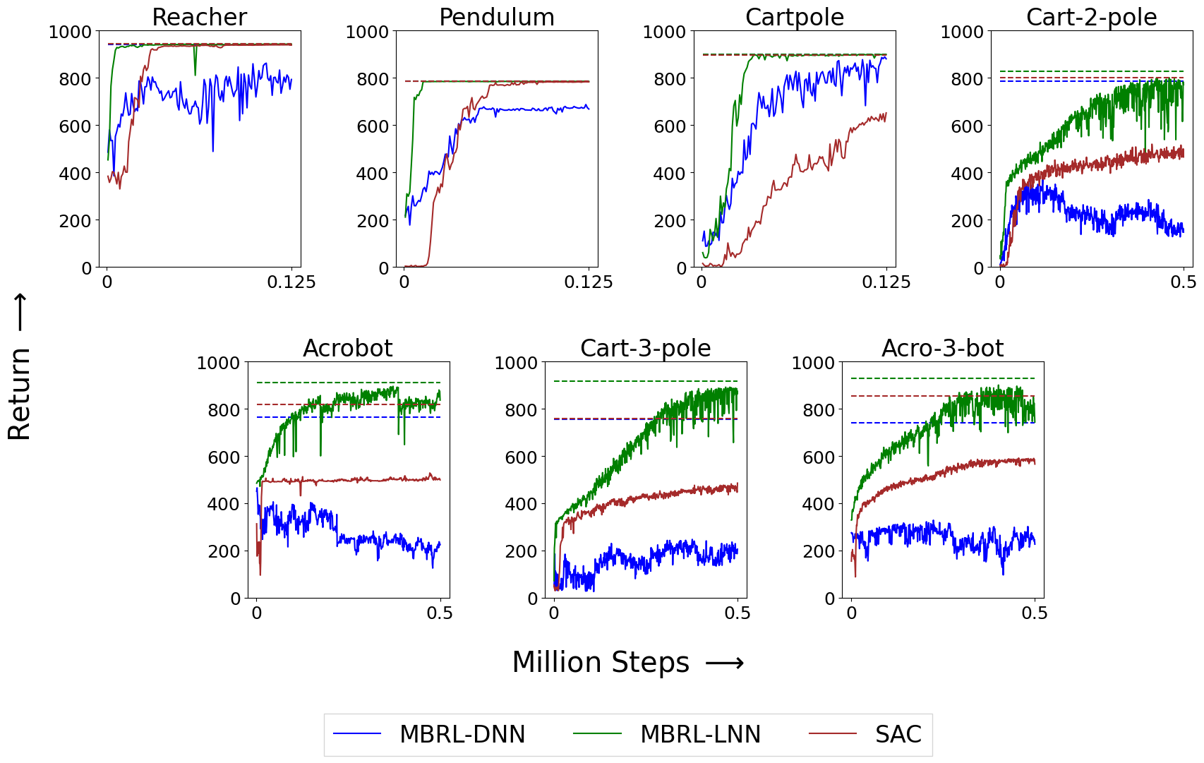
We show that, in model-based RL, model accuracy mainly matters in environments that are sensitive to initial conditions, where numerical errors accumulate fast. In these environments, the physics-informed version of our algorithm achieves significantly better average-return and sample efficiency. In environments that are not sensitive to initial conditions, both versions of our algorithm achieve similar average-return, while the physics-informed version achieves better sample efficiency.
We measure the sensitivity to initial conditions by computing the rate of separation of trajectories which start from nearby initial states, i. e., by computing the Lyapunov exponents. More specifically, we compute the finite-time maximal Lyapunov exponent. The sensitivity to initial conditions depends on factors such as the system dynamics, degree of actuation, control policy and damping.
We also show that, in challenging environments, physics-informed model-based RL achieves better average-return than state-of-the-art model-free RL algorithms such as Soft Actor-Critic, as it computes the policy-gradient analytically.
Videos
We show the behaviours learnt by our physics-informed model-based RL approach below.