Rigid body dynamics simulation

Introduction

We focus on the robotics domain, mainly robotic manipulators, although the same principles can be applied to other robotic systems. Robotic manipulators essentially undergo rigid body motion. For simplicity we assume that there is no friction or contacts. For such systems, it is easier to derive the equations of motion using Lagrangian or Hamiltonian mechanics rather than Newtonian mechanics. Conventionally, the Lagrangian approach is taken.

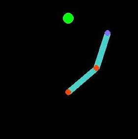
We consider a simple robotic manipulator with 2 dof commonly referred to as reacher. We assume that the robot is situated on the horizontal plane ie there is no gravity. We show how to simulate it from first principles.

Lagrangian Mechanics

These systems obey Lagrangian mechanics. Their state consists of generalized coordinates $\textbf{q}$, which describe the configuration of the system, and generalized velocities $\dot{\textbf{q}}$, which are the time derivatives of $\textbf{q}$. Let the motor torques be $\boldsymbol\tau$. The Lagrangian equations of motion are given by, \[\textbf{M}(\textbf{q}) \, \ddot{\textbf{q}} + \textbf{C}(\textbf{q},\dot{\textbf{q}}) \, \dot{\textbf{q}} + \textbf{G}(\textbf{q}) = \boldsymbol\tau\]

where, $\textbf{M}(\textbf{q})$ is the mass matrix, $\textbf{C}(\textbf{q},\dot{\textbf{q}}) \, \dot{\textbf{q}} = \frac{\partial }{\partial \textbf{q}} \big(\textbf{M}(\textbf{q})\, \dot{\textbf{q}} \big) \, \dot{\textbf{q}} - \frac{\partial }{\partial \textbf{q}} \big( \frac{1}{2} \, \dot{\textbf{q}}^{T} \, \textbf{M}(\textbf{q})\, \dot{\textbf{q}} \big)$ is the centripetal / Coriolis term and $\textbf{G}(\textbf{q}) = \frac{\partial \mathcal{V}(\textbf{q})}{\partial \textbf{q}}$ is the gravitational term, where $\mathcal{V}(\textbf{q})$ is the potential energy.

Derivation of M, C, G for Reacher

Below we show how to derive the mass matrix $\textbf{M}(\textbf{q})$, the centripetal / Coriolis term $\textbf{C}(\textbf{q},\dot{\textbf{q}}) \, \dot{\textbf{q}}$ and the gravitational term $\textbf{G}(\textbf{q})$ using Sympy, a symbolic library for Python.

from sympy import symbols,cos,sin,simplify,diff,Matrix,linsolve,expand,nsimplify,zeros,flatten
from sympy.utilities.lambdify import lambdify
from sympy.matrices.dense import matrix_multiply_elementwise
import dill as pickle
pickle.settings['recurse'] = True

def get_C_G(n,M,V,q,qdot):
    C = zeros(n)
    for i in range(n):
        for j in range(n):
            for k in range(n):
                C[i,j] += (diff(M[i,j],q[k])+diff(M[i,k],q[j])-diff(M[k,j],q[i]))*qdot[k]/2

    G = Matrix([diff(V,q[i]) for i in range(n)])

    return C,G
    
def derive():
    lambda_dict = {}
    n = 2
    m1,m2 = symbols('m1,m2')
    l1,l2 = symbols('l1,l2')
    r1,r2 = symbols('r1,r2')
    I1,I2 = symbols('I1,I2')
    g = symbols('g')
    q1,q2 = symbols('q1,q2')
    q1dot,q2dot = symbols('q1dot,q2dot')

    m = [m1,m2]
    l = [l1,l2]
    r = [r1,r2]
    I = [I1,I2]
    inertials = m+l+r+I+[g]

    q = Matrix([q1,q2])
    qdot = Matrix([q1dot,q2dot])
    state = [q1,q2,q1dot,q2dot]

    J_w = Matrix([[1,0],
                  [1,1]
                 ])

    angles = J_w * q

    V = 0
    M = zeros(n)
    J = []
    for i in range(n):
        if i == 0:
            joint = Matrix([[0, 0]])
            center = joint + (r[i])*Matrix([[sin(angles[i]),cos(angles[i])]])
            joints = joint
            centers = center
        else:
            joint = joint + l[i-1]*Matrix([[sin(angles[i-1]),cos(angles[i-1])]])
            center = joint + (r[i])*Matrix([[sin(angles[i]),cos(angles[i])]])
            joints = Matrix.vstack(joints, joint)
            centers = Matrix.vstack(centers, center)
        
        J_v = center.jacobian(q)
        # J.append(J_v)
        M_i = m[i] * J_v.T * J_v + I[i] * J_w[i,:].T * J_w[i,:]
        M += M_i
             
        V += m[i]*g*center[0,1]

    # print(cse([centers,joints,J_w]+J, optimizations='basic'))

    C,G = get_C_G(n,M,V,q,qdot)
    lambda_dict['kinematics'] = lambdify([tuple(inertials+state)],[centers,joints,angles],'numpy',cse=True)
    lambda_dict['dynamics'] = lambdify([tuple(inertials+state)],[M,C,G],'numpy',cse=True)
    
    with open("./env/reacher/robot.p", "wb") as outf:
        pickle.dump(lambda_dict, outf)

    print("Done")

if __name__ == '__main__':
    derive()

Simulation

To simulate the system, we numerically integrate the governing ODE. Below we list some commonly used numerical integration techniques. In practice, we use the RK4 method. RK stands for Runge-Kutta.

• RK1 / Euler integration

• RK2

• RK4

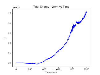
• Energy check

To verify the correctness of the simulation, we can plot the total energy as a function of time. We simply use a random policy.

Videos

We show a video of the simulation below. We use a pretrained policy, although a random policy could be used as well.

Code

You can find code used in this tutorial here, code.